Further Examples of Camera Design Using LUM

Jim Worthey • Lighting & Color Research • jim@jimworthey.com • 301-977-3551 • 11 Rye Court, Gaithersburg, MD 20878-1901, USA

Further Examples of
"Camera Design Using Locus of Unit Monochromats"

Five Examples for Comparison

The 5 examples are worked out in detail, and are consistent in their use of the "fit first" calculation method. As explained in the next few paragraphs, the fit first method is a simplified version of the method in "Camera Design Using Locus of Unit Monochromats". For an analysis of the Foveon X3 sensor, emphasizing the effect of the prefilter, read all of this page.

[Note for students of the tutorials in 2007 (Albuquerque) and 2008 (Portland, OR): the material below attempts to justify the "fit first" method, versus the method of the published paper from CIC 14. In the tutorial, we assumed that the Fit First method is best, with little discussion. If it works, why argue? I suggest that you enjoy the 5 examples above, and don't study the discussion below. JAW 2008 June 29.]

An Exception that Proves the Rule: Foveon X3 and Optional Prefilter

It is common in English to speak of "the exception that proves the rule." The word "prove" is used in an older sense, meaning to test the rule, to find its limitations.

The methodology of "Camera Design Using Locus of Unit Monochromats" is based on mathematical truths combined with practical assumptions about cameras:

Mathematical truths:
1. Any set of functions can be orthonormalized by the Gram-Schmidt method. It is always possible to find an orthonormal basis for the camera sensors. In fact, an unlimited number of orthonormal bases exist.
2. It is always possible to start by finding an "achromatic" function for the camera that is a best fit to the human achromatic function, commonly called y-bar. The camera's achromatic function can be a linear combination of its red and green sensors, or a linear combination of all 3 sensors.
3. The camera's Locus of Unit Monochromats is invariant. Any orthonormal basis will lead to an LUM for the camera with the same shape, but when it is plotted, it may have a random orientation with respect to the human LUM.
4. Any orthonormal basis will suffice in order to use the algebraic shortcuts that depend on orthonormality.

Practical assumptions. Of course these are only practical if they work out:
1. Frankly, many articles have discussed vision or cameras with a focus on curve-fitting, or "quality metrics". The orthonormal basis and the locus of unit monochromats are intended to go beyond curve-fitting. To this end, the 4-step method (in the paper, under the heading of "Implementation") makes minimal use of curve-fitting as an intermediate step.
2. In particular, the method assumes that the camera has well-defined red, green, and blue sensors. That assumption suffices for the paper's 2 examples: a Nikon D1 camera¹, and a proposed ideal sensor set designed by Shuxue Quan². For other cameras, the sensors may not fit the ideal of red, green and blue.

Discussion: For example, the Sony ICX282AKF array has 4 spectral sensitivities: yellow, magenta, green, and cyan. To bring such a sensor array into a comparison with human, a good starting point would be make a best fit to human orthonormal sensitivities by linear combinations of the 4 functions. That would be interesting, (and easy to do using Matrix R) but for now the point is this: To the extent that the camera sensors are other than red, green, blue, an unconstrained curve-fitting step will be needed in order to set up the comparison.

The curve-fitting step does not diminish the benefits of finding the camera's LUM, and an orthonormal basis. It just makes the process look more dull and ordinary.

Fit first method: With all that in mind, we now explore "the exception that proves the rule," the interesting case of the Foveon X3 sensor without and with a prefilter. It was found in preliminary work that the 4 steps of the CIC 14 paper gave the LUM of Foveon X3 poorly aligned with human LUM. Putting aside the 4 steps, the LUM for Foveon X3 was derived by a process that we can call "fit first." The fit first calculation is simpler than the 4 steps. The computer code looks like this:

Rcam = RCohen(rgbSens)

  CamTemp = Rcam*OrthoBasis

  GramSchmidt(CamTemp, CamOmega)

Here

rgbSens is a matrix whose
columns are the 3 camera sensor functions (in this case the Foveon
functions) .

Rcam

 is the projection
matrix based on the camera functions.

OrthoBasis

 is the 3
orthonormal
vectors for human, often called

Ω . CamTemp is then the best fit to OrthoBasis using a linear combination of the camera sensitivities. In general, the columns of CamTemp will not be an orthonormal set, so the Gram-Schmidt procedure is used to orthonormalize them. The orthonormal basis for the camera sensors is then CamOmega. That's the main result, and the camera's locus of unit monochromats is a parametric plot of the 3 columns of CamOmega.

Foveon X3 Sensor without Prefilter

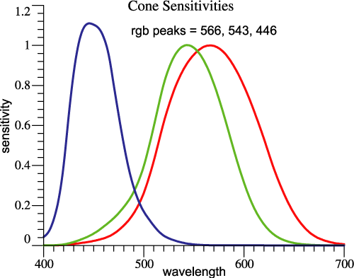
We now analyze the Foveon X3 sensor³, not applying the prefilter. The camera sensors are shown with human cone functions for comparison:

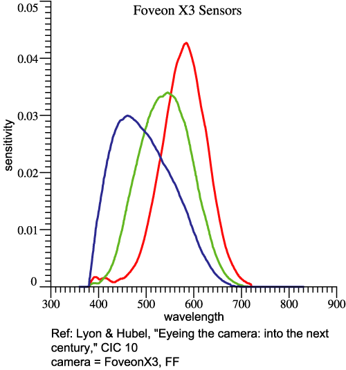
Human Eye	Foveon 3-Color Camera Sensor

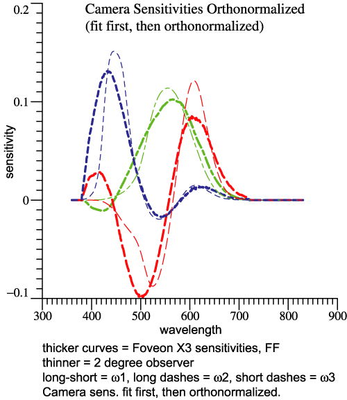
Collectively, the Foveon X3 functions are wider than the cone functions: they have substantial sensitivity in the vicinity of 400 nm and 700 nm. They show greater overlap than the camera functions in the article, which suggests that the Foveon sensor may show smooth wavelength discrimination through the green and blue-green, more so than the other cameras. To compare the Foveon X3 in detail to other sensors and the eye, we use the "fit first method" above.

We now graph two representations of the Foveon X3 color-matching traits: first the camera's native orthonormal basis; then a best fit to the 2º Observer orthonormal functions, using the camera functions.

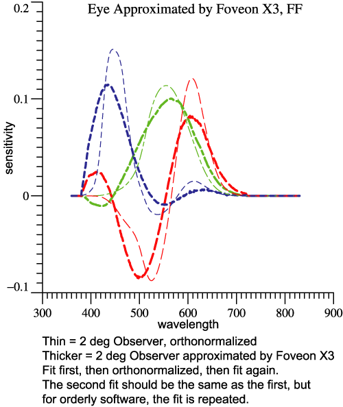
Native Orthonormal Basis of Foveon X3	Fit to Human Orthonormal Basis by Foveon X3 functions

Yes, these 2 graphs are nearly the same. The thinner curves are the same in both cases. On the right, the thicker curves are a best fit to the thin curves and are not an orthonormal set. For now we can say that these graphs are "for reference" and not try to parse their meaning too deeply. Recall that ω1 = achromatic; ω2 = red-green; ω3 = blue or blue-yellow if you wish. The locus of unit monochromats (LUM) is generated from the orthonormal basis by making a parametric plot in 3 dimensions. Each 3-dimensional plot is represented below by 2 projections. The thicker curves on the left above map to the black curves below, while the best fit functions (thicker curves on the right) map to the heads of the green arrows. The thin curves above are the human basis (2° observer) and generate the dashed red LUM below.

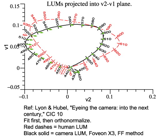
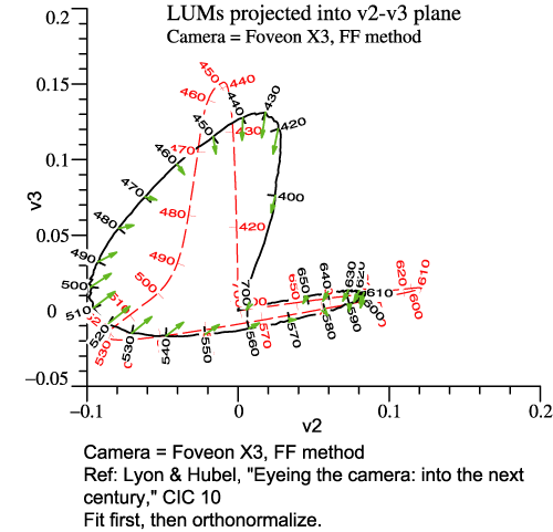
Red dashed = human LUM projected into v2-v1 Black solid = same projection of Foveon X3's LUM Heads of green arrows = fit to human by Foveon X3 functions, same projection.	Red dashed = human LUM projected into v2-v3 Black solid = same projection of Foveon X3's LUM Heads of green arrows = fit to human by Foveon X3 functions, same projection.
Click to see the LUM for Foveon X3 (without prefilter) graphed in 3 dimensions!

The orthonormal basis and LUM avoid double counting. We can make more definite statements based on the LUM, versus any tentative remarks based on the sensor functions r, g, b. Looking at either projection, the X3 responds smoothly to changing wavelength of a narrow-band light. Even considering the best fit transformation of the camera functions, the detailed response to wavelength differs from human. That is, there is obvious departure from the Maxwell-Ives criterion. In particular, there is a sort of excess sensitivity in the blue-green part of the spectrum, seen in the v2-v3 projection.

Foveon X3 Sensor with Prefilter

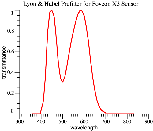
Same Foveon X3 Sensors as Before	This Prefilter³ Will Narrow the Functions and Reduce Overall Sensitivity in the Blue-Green Region

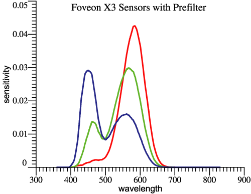
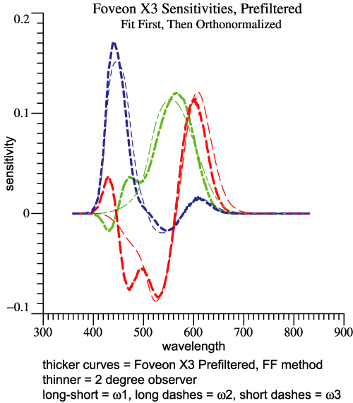
The filtered sensors are now seen in comparison to the unfiltered sensors (above), and cone sensitivities (to the right).

Foveon X3 Sensors Multiplied by the Prefilter Function³	Cone Sensitivities Consistent with 2º Observer

Applying the filter makes the sensors less like cone functions than before.

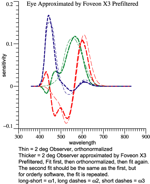
The thicker curves are the orthonormal basis for the Foveon X3 sensors with prefilter. The "fit first" method acts here to give a good alignment of the camera LUM with human LUM.	Fit to Human Orthonormal Basis by Pre-filtered Foveon X3 functions. The best fit was found from the orthonormal basis at left. The best fit should come out the same whether the orthonormal basis is derived by the "fit first" method or not. In fact, the fit first orthonormal basis was used.

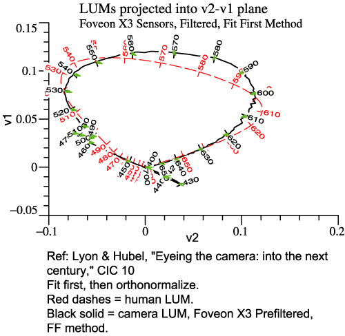
The locus of unit monochromats (LUM) is generated from the orthonormal basis by making a parametric plot in 3 dimensions. Each 3-dimensional plot is represented below by 2 projections. The thicker curves on the left above map to the black curves below, while the best fit functions (thicker curves on the right) map to the heads of the green arrows.

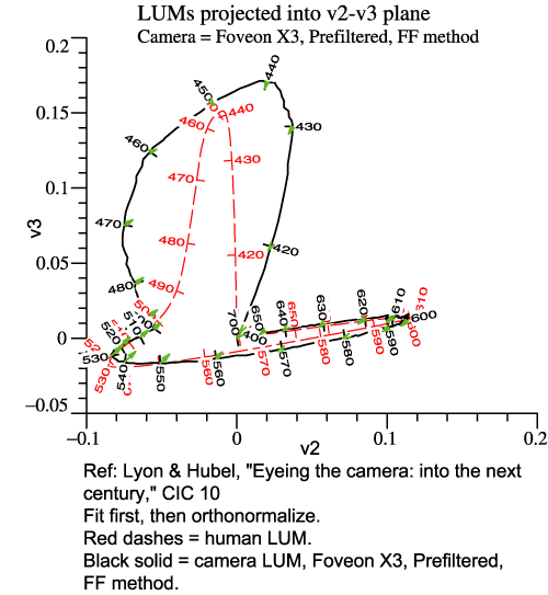
Red dashed = human LUM projected into v2-v1 Black solid = same projection of Prefiltered Foveon X3's LUM, found by fit first method. Heads of green arrows = fit to human by Prefiltered Foveon X3 functions, same projection.	Red dashed = human LUM projected into v2-v3 Black solid = same projection of Prefiltered Foveon X3's LUM, found by fit first method. Heads of green arrows = fit to human by Prefiltered Foveon X3 functions, same projection.
Click to see the LUM for Foveon X3 WITH prefilter, graphed in 3 dimensions!

Foveon X3 Sensor with and without Prefilter

An application of the LUM graphs might be to compare one camera to another. For example, how is the Foveon X3 with prefilter different from its sister system, the Foveon X3 without prefilter? The comparable graphs are now presented together. The LUM for the filtered system is right below that of the unfiltered:

Click to see the LUM for Foveon X3 (without prefilter) graphed in 3 dimensions!
Click to see the LUM for Foveon X3 with prefilter, graphed in 3 dimensions!

At this point, one could make some comment that the filtered version is or is not better, but let us gather more information. Recall Eqs. 15-18 in the CIC 14 paper. Extending the method to a 3-sensor system, let the camera sensors be the columns of array rgbSens, and CamOmega be the camera's orthonormal basis. Then

CamOmega = rgbSens*Y, where
Y = inv(CamOmega'*rgbSens) .

The tiny apostrophe, ', denotes matrix transpose. The transform Y can be found for any camera, and indeed for the eye itself.

2° observer himself

Foveon X3, no filter

Prefiltered Foveon X3

Y = inv(OrthoBasis'*rgbbar) =

0.0725	0.267	0.0376
0.0447	-0.310	-0.0543
0	0	0.138

Y = inv(CamOmega'*rgbSens) =

0.962	5.56	1.919
2.41	-6.98	-5.72
-0.783	1.61	5.84

Y = inv(CamOmega'*rgbSens) =

-0.544	9.40	2.67
5.61	-13.1	-7.86
-1.72	3.56	7.99

Column amplitudes =
0.0852 0.409 0.153

Column amplitudes =
2.71 9.06 8.40

Column amplitudes =
5.89 16.5 11.5

Obviously, Y is a 3×3 matrix and has nothing to do with the XYZ color system. The matrix elements are colorized so that the red entries (may look brownish) indicate the contribution of the red sensor to ω1, ω2, ω3. The green entries are the contributions from the green sensors, and so on for the blue entries. The 31 and 32 entries for 2° observer are zero because that was the intention in creating the orthonormal basis: no blue contribution to ω1, ω2. If those entries are small for a camera, it means that the camera is like the eye, in the sense of the "practical assumptions" above. The column amplitudes are the root of the sum of the squares, and relate to noise. The eye can't easily be compared to the cameras. For the 2 Foveon examples, we can see that the gains are increased when the filter is used, amplifying noise for a comparable signal. An enemy of a clean signal would be similar inputs multiplied by large gains and then subtracted. Without pursuing the analysis to its algebraic bitter end, we can see that such an effect would show up here.

Observation: The method in the CIC 14 paper is based on the assumption that Y₃₁ and Y₃₂ are small for the camera. By contrast, the "fit first" method is completely general so long as the camera has 3 or more spectrally independent sensor types that can be fit to the human orthonormal basis. Suppose that one were to write a general computer program for use by camera engineers. It might be best to

calculate all cameras by the "fit first" method, which is really simpler,
then also calculate the matrix Y for each camera,
and present it in colorized form as above.

Prime colors: The Foveon X3, with and without the prefilter, can be compared to the 2° observer on the basis of prime color wavelengths:

Prime Color λs	red	green	blue
2° observer	603	538	446
Foveon X3	587	510	430
Foveon X3, Prefiltered	591	541	442

The prefilter moves the prime colors closer to the values for the 2° observer. Because the camera LUMs are smooth, the prime colors are probably a good measure of color fidelity. The meaning of the prime color numbers would be less clear if the camera LUMs were irregular.

Disclaimer: In an online discussion, one colleague criticized the CIC 14 paper, pointing out that "colorimetric reproduction" may not be preferred. It is difficult to write about the Maxwell-Ives criterion without implying that it is a goal of camera design. However, the methods presented compare any camera's color-matching properties to those of the eye and other cameras, in a detailed and objective way. The designer can do what he wants. The comparison of LUMs could be used along with other methods, such as the mapping of a population of object colors; the object colors can be mapped in Cohen's space in diagrams similar to those I've made for the study of color rendering.

References
1 DiCarlo, Jeffrey M., Glen Eric Montgomery and Steven W. Trovinger, “Emissive chart for imager calibration,” Proceedings of the 12th Color Imaging Conference: Color Science and Engineering, Scottsdale, AZ, USA, November 9-12, 2004. Published by IS&T, Springfield, VA 22151, http://www.imaging.org.
2 Quan, Shuxue, Evaluation and optimal design of spectral sensitivities for digital color imaging, Ph. D. dissertation, Rochester Institute of Technology, 2002.
3 Lyon, Richard F. and Paul M. Hubel, "Eyeing the Camera: into the Next Century," Proceedings of the 10th Color Imaging Conference: Color Science and Engineering, Scottsdale, AZ, USA, November 12-15, 2002. Published by IS&T, Springfield, VA 22151, http://www.imaging.org.