| 0 |
Jump directly to
program
listings.
|
|
|
1
|
On
this web site,
the
phrase
"vectorial
color" denotes
a set of
methods in
which lights
are
represented by
vectors in the
color space
developed by
Jozef Cohen.
The vectors
are
tristimulus
vectors, based
on
the
orthonormal
color matching
functions. The
goal is to
make better
use of
existing
color-matching
data.
Whether the 10°
data are
better
than the 2°
data, or new
experimental
data are
needed, those
are separate
questions. You
choose
your data,
and the
vectorial
methods will
help to make
use of them.
The
starting point
for
vectorial
color is to
take existing
color
matching
functions,
such as
the 2°
observer
functions, and
add and
subtract them
to make
orthonormal
color matching
functions. The
"adding and
subtracting"
is done by
matrix algebra
and
in one step
uses the
well-known
Gram-Schmidt
method of
orthonormalization.
The purpose of
this web page
(as of 2006
June) is
to present a
few code
fragments and
short working
routines, to
show how
the work is
done. With
regard to some
methods, such
as
Gram-Schmidt,
it
is easier to
write a
program than
to describe
the method in
words and
symbols.
I do all my
calculations
in a
science-programming
language
called O-Matrix, which
allows matrix
operations to
be written as
easily as
operations on
scalars. If a
and b
are matrices
previously
created,
one can write
c
= a*b
to
right-multiply
a
by b.
The matrix c
need not be
declared or
dimensioned in
advance. In
short, steps
that are
simple in
concept remain
simple in
the
computer
program.
Another
language
similar to
O-Matrix is
Matlab. The
O-Matrix
manual exists
only as web
pages, and you
can view a
version on
their
web site.
If you would
like to
discuss color
calculations,
or request
more
details,
please contact
jim@jimworthey.com
, or call
301-977-3551
in the USA.
|
|
|
|
2
|
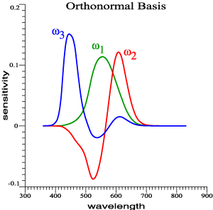
Suppose
for a moment
that
the
orthonormal
color matching
functions have
been found.
For the 2°
observer, they
are as graphed
above.
Conceptually,
they can be 3
column
matrices,
ω1, ω2, ω3.
The three
column vectors
can be grouped
together in an
N×3
matrix, where
N is the
number of
wavelengths:
Ω =
[ω1 ω2
ω3] .
This
is the kind of
notation used
in the
articles, with
the Greek
letters,
big and little
omega.
For
programming,
it is
convenient to
call Ω
something like
OrthoBasis:
Ω →
OrthoBasis
.
If
an individual
vector is
needed, it can
be referred to
in O-Matrix as
OrthoBasis.col(j), where j
= 1, 2, or 3
as needed. The
notation
".col(2)"
selects the
second column
of a matrix,
for example.
Now suppose
that D65 is a
column vector
representing
the spectrum
of
standard
daylight, D65.
We wish to
calculate its
tristimulus
vector,
which can be
called V65.
Then
V65
=
OrthoBasis'*D65
.
That
line of code
is in a larger
font to be
sure that you
can see the
apostrophe
after
OrthoBasis. It
indicates
matrix
transpose.
Using the
proper
notation then,
the
tristimulus
vector of any
light can be
found
in one line of
computer code.
In order to do
the operations
of
colorimetry by
matrix
operations,
one must align
the functions
of
wavelength
properly: they
must have the
same number of
elements and
the
same
wavelength
domain.
|
 |
|
|
3
|
In
the visuals of the 2004
talk,
"Color
Matching with
Amplitude not
Left Out," or
in the new
unpublished
article,
"Vectorial
Color," the
idea of
orthonormal
color matching
functions is
developed
step-by-step.
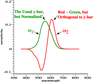
It is logical
to have one
all-positive
function, and
to let
that be an
achromatic
function that
is
proportional
to the usual
y-bar.
But the
achromatic
function can
be normalized.
Suppose that
ybar is
usual 2°
observer
function. Then
a code
fragment will
show the
steps:
prod
= ybar'*ybar
omega1
=
ybar/sqrt(prod)
.
Again
the apostrophe
denotes matrix
transpose.
sqrt(prod) is
then the
vector length
of ybar.
Dividing ybar
by its length
gives omega1,
a column
matrix
proportional
to ybar,
but with
length = 1. To
verify,
print
omega1'*omega1
.
The
result should
equal one.
Now
suppose that
red is
a
red cone
sensitivity
function. We
know that
omega1 is a
sum of red and
green, with
certain
proportions.
To make an
opponent
function
orthnormal to
omega1, we
subtract from
red the
projection of
omega1
onto
red, then
normalize:
omega2
= red -
(red'*omega1)*omega1
prod
=
omega2'*omega2
omega2
=
omega2/sqrt(prod)
In
normal
programming
fashion, the
array omega2
holds an
intermediate
matrix, then
the final
answer. The
steps above
illustrate the
method of
Gram-Schmidt
orthonormalization.
The following
O-Matrix
routine
calculates an
orthonormal
set from the
columns of any
matrix:
GramSchmidt(given, orthonorm)
.
The link will bring
up a text file
containing the
program. To
run it, you
must save the
text in a file
called
GramSchmidt.oms.
Calling the
Gram-Schmidt
routine
by the
following
steps will
create
OrthoBasis:
given = [ybar,
red, blue]
NumCols = 3
NumRows =
rowdim(given)
OrthoBasis =
zeros(NumRows,NumCols)
GramSchmidt(given,
OrthoBasis)
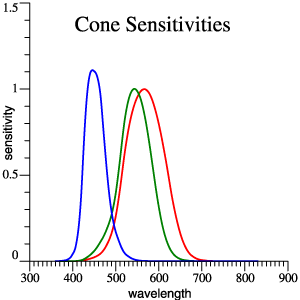
It is assumed that
there is a set
of cone
functions
{red, green,
blue} that are
linear
combinations
of the usual
xbar, ybar,
zbar of the 2°
observer, and
indeed that
ybar is a
linear
combination of
red and green
only. For
background,
see the Vectorial Color
manuscript,
especially the
appendices and
Figure 1.
Also see item
4 below.
|
 |
|
|
4
|
Just
above, and in
Figure 1 of the Vectorial
Color
Manuscript,
reference is
made to cone
sensitivity
functions
that are
linear
combinations
of the usual 2°
observer. I
take
the idea from
Guth, who
borrowed it
from Smith and
Pokorny.
Guth's
formula for
the cone
functions is
recalled in
Appendix A of
the "Render Calc" article.
Taking the
matrix
transpose of
that version,
including a
transposed
version of the
square
matrix, we can
write in
O-Matrix:
M1 = { [0.2435,
-0.3954, 0],
...
[0.8524,
1.1642,
0], ...
[-0.0516, 0.0837,
0.6225] }
rgb = xyzbar*M1
The
columns of
xyzbar are
assumed to be
the 2°
observer
functions.
That is xyzbar
= [xbar, ybar,
zbar] . The
actual data are here, or can
be obtained
from www.cvrl.org
. For my work,
I store most
spectral data
in a
particular
format that
is convenient,
but here the xyzbar data are
lumped in one
file,
just to show
that they're
available.
To get Guth's
1980 opponent
model directly
from xyzbar,
M3
=
{[0, 0.7401,
-0.0061], ...
[0.9341,
-0.6801,
-0.0212], ...
[0, -0.1567,
0.0314] }
atd =
xyzbar*M3
OrthoBasis =
zeros(NumRows,NumCols)
GramSchmidt(atd,
OrthoBasis)
The
result is the
same
orthonormal
basis as in
item 3. The
result should
also check
against this
file.
|
 |
|
|
5
|
Matrix
R.
Let A be a
matrix whose
columns are
three linearly
independent
vectors,
such as three
color matching
functions. For
example, A
could be the
usual 2°
observer
functions.
Then in
O-Matrix,
projection
matrix R can
be found by
Cohen's
formula:
A
= xyzbar
R =
A*inv(A'*A)*A'
In the
special case
that the
columns
of A are an
orthonormal
set, for
example if A =
OrthoBasis,
then A'*A
is an identity
matrix. Its
inverse is
also an
identity
matrix and one
may write for
this special
case only,
R
=
OrthoBasis*OrthoBasis'
An
O-Matrix
function can
be used:
Matrix R is a large
matrix. For
example, if A
indeed
contains the
2°
observer
functions at 1
nm intervals
and wavelength
domain 360 to
830
nm, then R has
dimensions 471×471, meaning that it
has 221841
elements and
in double
precision (8
bytes per
floating point
number), it
occupies
1774728 bytes.
On modern PC
hardware, this
storage
space and the
time to
calculate R
are absolutely
not a concern.
However, it is
not helpful to
print out the
matrix on
paper. On my
PC,
the time to
calculate
a 471×471 matrix R by
function
RCohen() is
about 13
ms.
|
 |
|
|
6
|
Putting
Matrix R to
work.
The
projection
matrix R can
be viewed in 2
ways. For
routine use of
the
orthonormal
basis, matrix
R is not
needed at all.
Matrix R can
be
considered as
background
information,
as the proof
that the
locus of unit
monochromats
has an
invariant
shape,
independent of
the
coordinate
system. The
orthonormal
basis is a
shortcut for
creating
color vectors
without using
matrix R
itself.
On the other
hand, matrix R
can be a
practical tool
for
curve-fitting
problems that
arise in
relation to
color. If
matrix A
contains any
1, 2, 3, or
more linearly
independent
vectors, then
the
projection
matrix R can
be found. Then
if any vector
X (with the
same
number of rows
as A or R) is
multiplied by
R, the result
is the
projection of
X into the
column space
of A. That is,
Xstar = R*X,
where
Xstar is the
projection. An
alternate
wording is
that Xstar is
the
least-squares
best fit to X,
using the
columns of A.
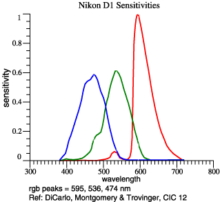
On the right
are
graphed the
red, green,
and blue
sensitivities
of a digital
camera. In
analyzing and
applying this
color
sensor, one
might wish to
find a linear
combination of
the camera's
red
and green
sensitivities
that best
approximates
the human
achromatic
sensitivity.
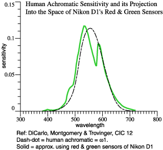
An alternate
statement of
the same goal
is that we
wish to
project the
human
achromatic
function into
the the vector
space of the
camera's red
and green
sensors. Let
the camera's
sensitivities
be
called redcam,
greencam,
bluecam. Then
Arg
= [redcam,
greencam]
Rrg
= RCohen(Arg)
achcam
=
Rrg*OrthoBasis.col(1)
Column matrix
achcam is then
the best
approximation
to the
human
achromatic
function, OrthoBasis.col(1),
by a
combination of
redcam and
greencam. The
lower graph
shows achcam
compared to
OrthoBasis.col(1).
More steps
would be
needed for the
complete
analysis of a
camera. At
this moment,
in 2006 June,
I am preparing
a paper on
that topic,
with a
co-author. For
now, the topic
is
calculation.
The methods on
this page
can be used
for such steps
as these:
- Find an
orthonormal
basis for the
camera itself.
By combining
those
functions,
find the
camera's locus
of unit
monochromats.
- Find the best fit to
all 3 human
sensitivities
by the camera
sensitivities.
The actual
programming is
reduced to a
few steps, and
the problem
becomes one of
concepts: what
do you want
the camera to
do?
|
|
|
|
7
|
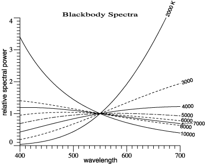
Blackbody
spectra can be
calculated by
this routine:
blackbody(Tkelvin,
descrip,
LamLoHi, vec)
.
Tkelvin = Kelvin
temperature of
the blackbody
descrip = a character
array that
will be set
with a
description of
this light
LamLoHi = the domain
of wavelength,
such as [360,
830].
vec = the result, a
column matrix
containing the
blackbody
spectrum
The blackbody
spectrum is
adjusted so
that it = 1 at
555 nm. In
this case,
LamLoHi
is an input,
set by the
calling
program. My
programs are
inconsistent
about this,
whether
LamLoHi must
be set by the
calling
routine. Since
I want all
spectra to
have the same
domain, the
domain
is often set
by a global
variable.
|
 |
|
|
|
|
|
|
|
|
|
|
|