Worthey Visuals for Seattle

Talk Itself Starts Here

Timeline of Science and Lighting

I developed an extended chronology with citations and details, from which Nicholas Worthey developed the graphical timeline above. Please enjoy the extended chronology and share any comments.

"A Mixture of Monochromatic Yellow and Blue Light"

The Illuminating Engineering Society of North America was founded on January 10, 1906. An early thought-provoking analytical idea appeared in 1912 in the Transactions of the Illuminating Engineering Society. [Herbert E. Ives, "The relation between the color of the illuminant and the color of the illuminated object," Transactions of the Illuminating Engineering Society 7:62-72.(1912).] In a passing remark, Herbert Ives noted

“It is, for instance, easily possible to make a subjective white, as by a mixture of monochromatic yellow and blue light. A white surface under this would look as it does under ‘daylight’ but hardly a single other color would.” -- H. E. Ives

An illustration from that article can be marked up to illustrate what he meant. From Isaac Newton's color article, we may take the idea that most white lights contain all colors of the spectrum. Ives applied a more detailed understanding, perhaps from Maxwell and from his father Frederic Ives, that a mixture of two narrow bands, yellow and blue, will be perceived as white. Below is Fig. 1a from that article.

A figure from 1912 with
additional lines added.

The black lines are Ives’s original drawing, while the orange and blue are added to represent his “mixture of monochromatic yellow and blue light.” Color vision is trichromatic, but monochromatic yellow stimulates two receptor systems because of the large overlap of the red and green sensitivities.

Ives Took a Scientific Approach.

Ives’s scientific insight:

The simple example is based on the facts of color vision.
The two-bands light anticipates issues with commercial lights that came later.


A modern version of red-green-blue.	Example like Ives's: Papers lose their color when 4002 K blackbody is replaced by a 2-band light of the same chromaticity.

2-bands Issue Since 1912

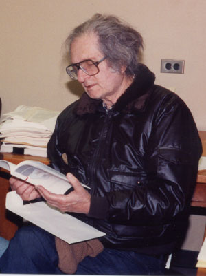
William A. Thornton
1923-2006

2-bands light from Thornton and
Chen article.

A figure from Thornton, William A. and E. Chen, “What is visual clarity?” J. Illum. Eng. Soc. 7(2):85-94 (January 1978).

In the 1970s, Bill Thornton studied the idea of 3-band lamps. He re-discovered Herbert Ives's idea, figure at left.

In the 1980s and since, Worthey has expanded on the two-bands idea, noting that many commercial lights shrink red-green contrasts among objects. See figure above.

The 1965 "Color Rendering Index" ignored the overlap of receptor sensitivities and the issue of the two-bands light. The current CRI still ignores the issue.

Why Is it Hard to Discuss Vision and Lighting?

Illustration developed by Nicholas Worthey. Chimpanzee photo by Thomas Lerch.

The normal process of seeing is effortless. Talking about it is harder.

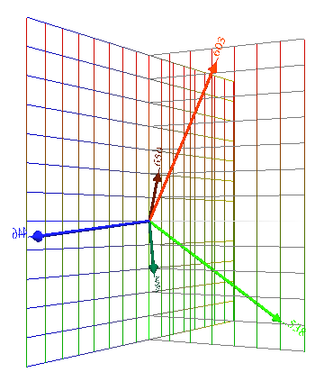
Vectorial Color Overview (part 1)


Narrow-band lights of equal power map to vectors with different amplitudes and directions.	Colored lights add vectorially. In this figure, equal-power components add to make the so-called Equal Energy Light.

Vectorial Color Overview (part 2)


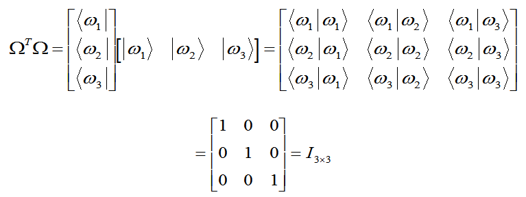
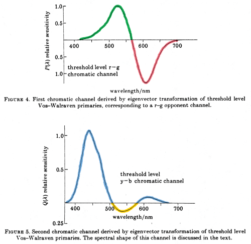
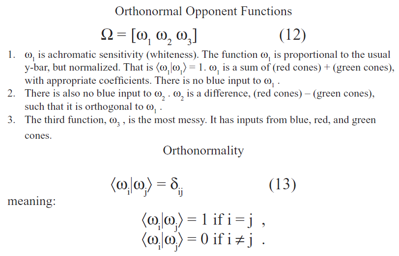
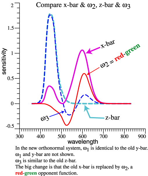
Starting with a light (an SPD), to find its 3-vector, we need these Orthonormal Opponent Color Matching Functions.	For convenience, the functions ω₁, ω₂, ω₃ become the columns of matrix Ω .

Vectorial Color Overview (part 3)

Vectorial Color was not invented to solve a single problem.
It emerged from past research, including
Ewald Hering's opponent-color ideas.
Quantitative results from Smith & Pokorny and quantitative opponent model of Sherman Lee Guth.
Thornton's analysis leading to the Prime Colors, the least-power primaries.
Analysis by Michael H. Brill.
Information theory analysis by Buchsbaum and Gottschalk.
Worthey's research on applications of Guth's opponent model, 1980 version.
And especially the formulas and theorems of Jozef B. Cohen.

Jozef B. Cohen
1921-1995

Legacy Understanding

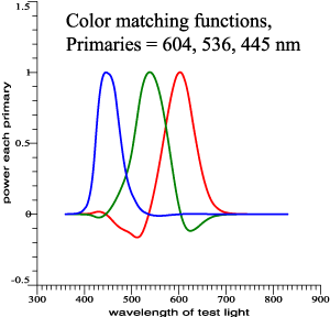
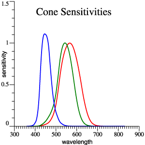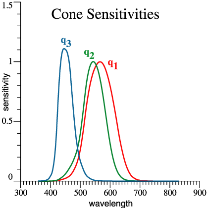
Fictitious but realistic color-matching data.			Cones, red, green and blue.
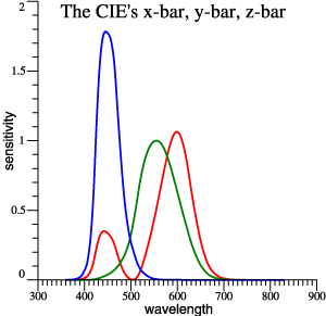
Traditional x-bar, y-bar, z-bar			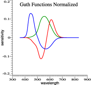Guth's 1980 model, normalized. Achromatic function is proportional to y-bar.
Linear transformations of color-matching data predict the same matches. This is Figure 1. < The only numbered figure! >

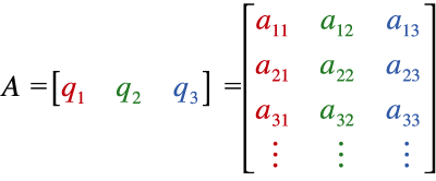
3 functions become the columns of a matrix:

	(Eq. 1)
A set of color matching functions, CMFs, become the columns of a matrix A. Or, if you like, the columns of A are a set of linearly independent functions, usually 3 functions.

SPD as a Column Vector

The spectral power distribution of any light can be written as a column vector L₁. It is then summarized by a tristimulus vector V,

V = A^T L₁ . (2)

Light L₁ is a color match for light L₂ if

A^T L₁ = A^T L₂ . (3)

Refer again to the Figure 1. If Eq. (3) holds for one set of CMFs A, then it will hold for the other sets. That much is standard teaching.

4 lights that approximately match in color.

Color Mixing Experiments: Choice of 3 λs .

Wavelength of the test light -->	For a color-matching experiment, different sets of 3 primary λs can be used. However, Wright and Guild both used red, green, and blue primaries. The wavelengths are not really arbitrary. The mixing of 3 primaries is a model for color displays. The graph at left shows that Guild and Wright used different primaries, and got different results.
	Thornton found: The color matching functions tend to peak at certain fixed wavelengths, despite a change of primaries. The peaks occur at certain λs , the prime colors. Prime color primaries run the experiment at minimum power.
For the 2° Observer, the prime colors are 603, 538, and 446 nm. Since they are based on a minimum-power criterion, they are "prime" candidates for RGB video primaries, subject to further study.

Strongly Acting Wavelengths

Thornton began by asking “Which wavelengths act strongly in mixtures?”

By various calculations, he found 3 strongly acting wavelengths.

Later he realized that the basic color mixing experiment measures “action in mixtures.”

Strongly acting wavelengths are not a weird new idea. They are an old idea that was never put into words.

Some Credit to Tom N. Cornsweet

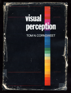In his 1970 Book, Tom Cornsweet used vector diagrams to discuss overlapping receptor sensitivities.

Jozef Cohen and the Fundamental Metamer

Jozef B. Cohen's Book

Cohen sought an invariant presentation of color mixing facts.

Consider any light L(λ).
L*(λ) = the Fundamental Metamer of L(λ) = the projection of L(λ) into the space of color-matching functions, CMFs.
Start with L(λ) , and with a set of 3 CMFs. Find the linear combination of the CMFs that is a least-squares best fit to L(λ) . That is the projection. That's the fundamental metamer.
L*(λ) is invariant. For example, start with any of the 4 sets of CMFs at the right. L*(λ) comes out the same.
Cohen found an easy method to obtain L*(λ) .
Cohen's method for finding L* lead him to other ideas.

4 presentations of
the same color-mixing facts.

4 Legacy Graphs

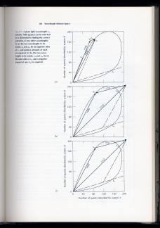
Examples of Fundamental Metamers.

4 items: Fundamental metamer of a narrow band. 1 item: Fundamental metamer of D65. Fundamental metamer is always a smooth curve.

Joe Cohen's easy method: Matrix R

Cohen needed a way to find a fundamental metamer L* . As before, A is a matrix whose columns are a set of CMFs,
	. (1)
Given L and A, we want to find L* . Now a student might look up Moore-Penrose pseudo-inverse and get a numerical answer L* with that . Lucky for us, Cohen did not have Wikipedia and solved the problem for himself, which led him to more ideas. Long story short, Cohen's method: L* = R L , (2) where R = A(A^TA)⁻¹A^T . (3)

Matrix R, continued.

Fun Facts about Matrix R

Cohen often used "Matrix R" as the name for a broad area of research.
Matrix R is a large square array. If the domain of λ has 471 steps, then R is a 471 x 471 matrix. That causes no trouble, but don't try to print it.
Matrix R itself is invariant. Sets of CMFs that are different (but equivalent) lead to the same big array R.
Matrix R is a projection matrix. It is symmetrical.
The columns (or rows) of R are the fundamental metamers of the spectrum.
In other words, the columns of R, interpreted as 3-vectors, trace the Locus of Unit Monochromats, the LUM.
It is easier to explain and draw the LUM using the orthonormal basis.
Some proofs about R are on my web site, as well as in Cohen's articles and book.

Fundamental Metamer Example.

At left, the blue curve shows L = D65. The purple curve is L*, the fundamental metamer of D65. The two curves are metamers in the ordinary sense. L*, a linear combination of CMFs, is found by:

L* = RL . (4)

Eq. (4) has '=' and not '≈' because L* by definition is the least-squares approximation.

So that’s Jozef Cohen’s
Highly Original Contribution.

Now a few screens above,
We were talking about vectors...

Cohen References:
Cohen, Jozef, “Dependency of the spectral reflectance curves of the Munsell color chips,” Psychonom. Sci. 1, 369-370 (1964).

Cohen, Jozef, Visual Color and Color Mixture: The Fundamental Color Space, University of Illinois Press, Champaign, Illinois,
2001, 248 pp. <2014 update: book is out of print. Publisher has allowed a version to be posted on Google Books. Check it out! >

Orthonormal Opponent Color Matching Functions.

In the past—since 1980—I had used opponent color algebra. In 2003, I discovered that a set of Orthonormal Opponent Color Matching Functions is closely related to Cohen's Matrix R, fundamental metamers, and the vector diagrams that he made.

The functions are easy to generate, or can be found at
http://www.jimworthey.com/orthobasis.txt .
I first generated them by applying Gram-Schmidt orthonormalization to Guth's 1980 functions.

Orthonormal Opponent Color Matching Functions: Description.

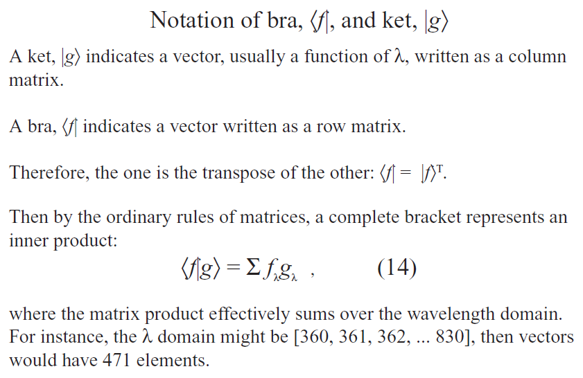
Bra and Ket Notation

Working Class Summary

Although many clever ideas (from Cohen, Guth, Thornton, Buchsbaum, etc.) guided its development, in the end the orthonormal basis is not radically new:

ω₁ is proportional to old-fashioned y-bar (not shown). So ω₁ is not new.

ω₃ is similar to the old z-bar, which is essentially a blue cone function.

In the XYZ system, x-bar is an arbitrary magenta primary. It is replaced in the new system by ω₂ , a red-green opponent function.

An important feature of human vision is the overlapping sensitivities of the red and green cones. An opponent system confronts the issue of overlap. It re-mixes the red and green signals into ω₁ = red + green, and ω₂ = red - green.

Click to review graph of orthonormal basis
(Then use browser's back button.)

Fun with Matrices

Ω = [ ω₁ ω₂ ω₃ ] (12)
〈ω_i|ω_j〉 = δ_ij . (13)

Orthonormality, Eq. (13), can be expressed in matrix form:

(15)

or in short, Ω^TΩ = I_3×3 . (15)

If you multiply Ω and its transpose in the reverse order, you get a different interesting result:

ΩΩ^T = R . (16)

Eq. (16) is easily proved, but not right now. [Just substitute A = Ω in Eq. (3).]

Convenience of the Orthonormal Basis

To repeat,

Ω^TΩ = I_3×3

and

ΩΩ^T = R .

These simple facts make calculations easier. For details, see references [15] and [16] .
[15] James A. Worthey, "Vectorial color," Color Research and Application, 37(6):394-409 (December 2012).
[16] James A. Worthey, "Applications of vectorial color," Color Research and Application, 37(6):410-423 (December 2012).

Recall from a few screens above:

	Given light L, find its 3-vector V by a matrix multiplication. Ω is known and constant.
Starting with a light (an SPD), to find its 3-vector, we need these Orthonormal Opponent Color Matching Functions.	For convenience, the functions ω₁, ω₂, ω₃ become the columns of matrix Ω .

Meaning of Tristimulus Values

v₁ = whiteness = achromatic or black-white dimension
v₂ = redness or greenness
v₃ = blueness or yellowness
So, we can say that the tristimulus values have intuitive meaning.
But that's not all.

|L*〉 = v₁|ω₁〉 + v₂|ω₂〉 + v₃|ω₃〉

If we express the fundamental metamer L* by an orthonormal function expansion, the tristimulus values are the coefficients. The same values have mathematical meaning.

Graphing a Vector

So, we can calculate one vector from the origin.

5 Vectors

Or five vectors from the origin.

5 Vectors Added

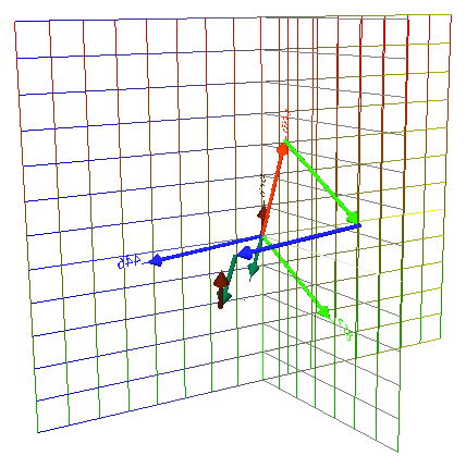Or add some vectors vectorially. That is they add tail to head.

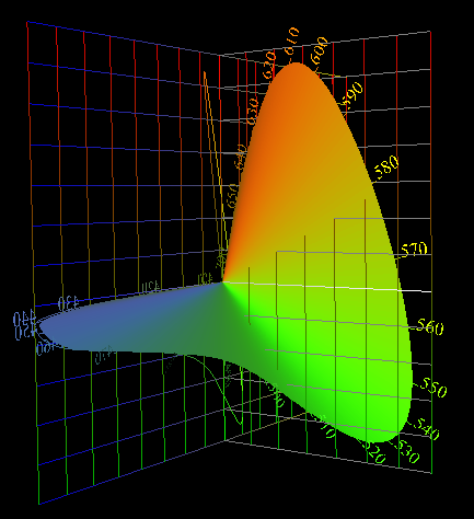
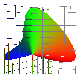
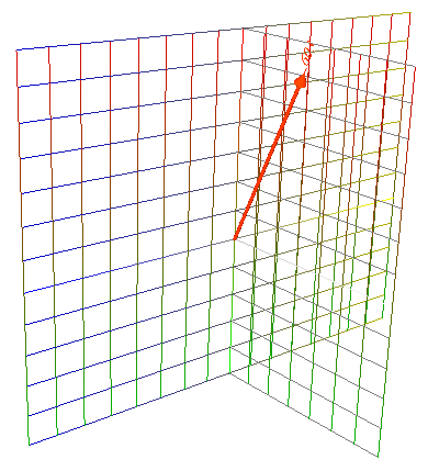
Locus of Unit Monochromats

Narrow-band light, wavelength λ.
Light has unit power. <A leap forward by Cohen>
Step λ through the spectrum.
Plot vectors.
The result is a spectrum locus in 3 dimensions,
"The Locus of Unit Monochromats," the LUM.

In Cohen's original presentation, the vectors are fundamental metamers. Now recall

The columns of Omega are the
orthonormal fns.

The 3-vectors of the LUM are the rows of Ω .
Simple!

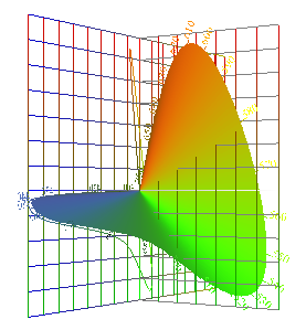
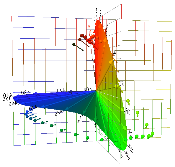
Locus of Unit Monochromats (continued)

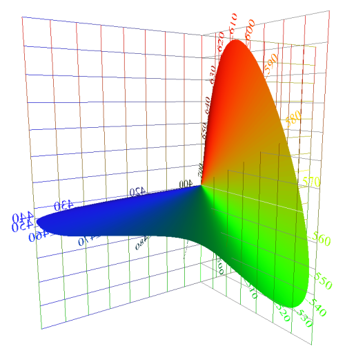I sometimes show the Locus of Unit Monochromats (LUM) by a surface. The locus is really the curve along the edge of the surface.

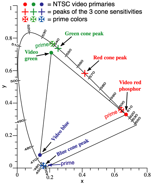
Wavelengths of Strong Action

The NTSC phosphors are approximately at Thornton’s Prime Colors, 603, 538, 446 nm.

Wavelengths of strong action in mixtures, nm.
2º Observer
longest vectors =	445	536	604
prime colors =	446	538	603
10º Observer
longest vectors =	445	535	600
prime colors =	445	536	600

For practical purposes, the wavelengths of the longest vectors are the same as the prime colors, and about the same as the NTSC phosphors.

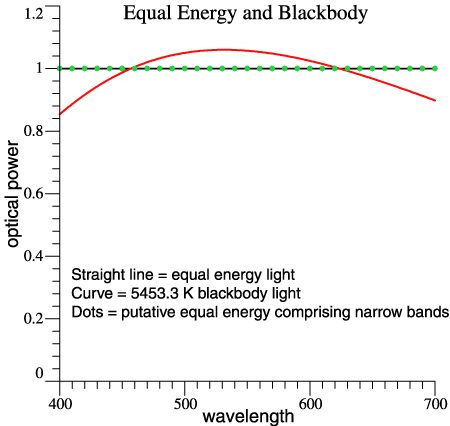
Composition of a White Light

The so-called "equal energy light" is one that has constant power per unit wavelength across the spectrum, indicated by a solid black line in the figure at the right.

The straight-line spectrum is similar to a more realistic light, 5453 K blackbody (or 5500 if you like).

Now assume an equal-energy light that packs all of its power at the 10-nm points, 400, 410, ... , shown by the green dots.

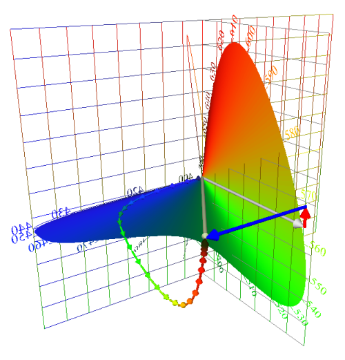
Composition of a White Light (continued)

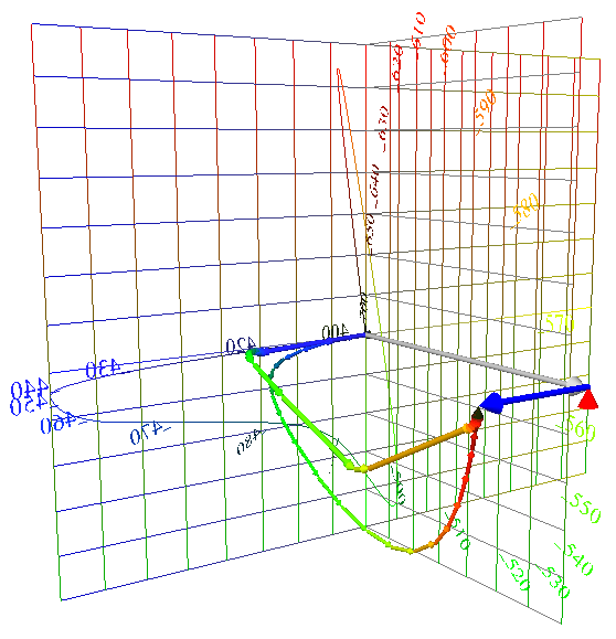
At right, each band contributes an arrow: blue, blue ..., blue-green, blue-green ... green ... green-yellow ... orange ... red. Added tail to head, the arrows sum to the "equal energy" white.

The chain of 31 arrows makes progress towards blue, then swings in the green direction, then back towards red.

The red and green components of a white light cancel each other out. They need to be present in order to reveal red and green objects. This is the issue from Herbert Ives in 1912.

Miniature
sketch of Ives idea.
Bell pepper photo by Kham Tran

Skip one item

Opponent Colors and Information Transmission

In 1983, Buchsbaum and Gottschalk derived an opponent-color system to optimize information transmission. They started with cone functions and got a result like the orthonormal basis Ω .

It is perhaps intuitive that Ω is helpful for engineering work because redundancy is taken out. The Buchsbaum and Gottschalk result supports the use of Ω for image compression and propagation-of-errors, for example.

[Gershon Buchsbaum and A. Gottschalk, “Trichromacy, opponent colours coding and optimum colour information transmission in the retina,” Proc. R. Soc. Lond. B 220, 89-113 (1983).]

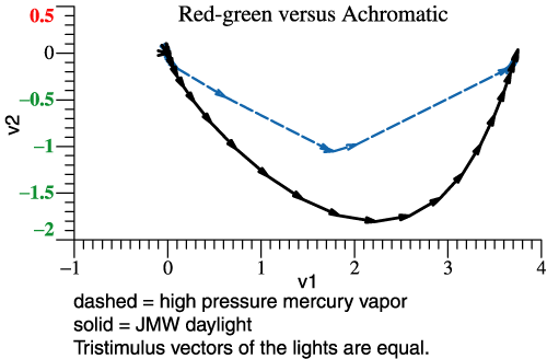
Some Lights Have Less Red and Less Green

A white light has net redness or greenness that is small or zero. The same white point can be reached by different lights in different ways.

SPDs of 2 lights are plotted at right. The black line is High Pressure Mercury Vapor light, while the blue is JMW Daylight, adjusted to have the same tristimulus vector. (Yes, that means they are matched for illuminance and chromaticity.) The wavelength domain is chopped according to the dashed vertical lines. The wavelength bands are 10 nm, except at the ends of the spectrum, with most bands centered at multiples of 10 nm. If one light then multiplies the columns of Ω, those products could be graphed as a distorted LUM, but we skip that step.

Mercury light
spectrum and daylight spectrum.

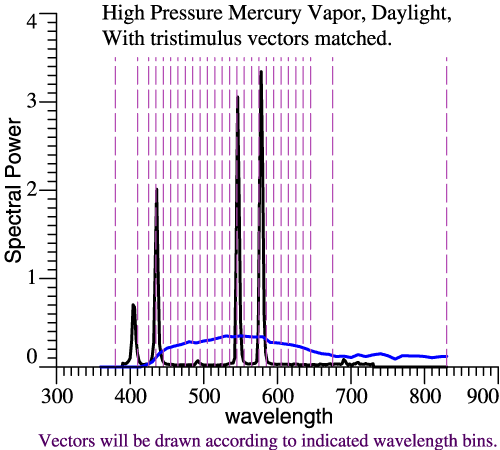Instead, the color composition of each light will be graphed as a chain of vectors.

Comparing Color Composition of Lights

Now the same two lights are compared in their vector composition. The smooth chain of thin arrows shows the composition of daylight. Slightly thicker arrows show the mercury light. The mercury light radiates most of its power in a few narrow bands, leading to a few long arrows that leap toward the final white point. Compared to “natural daylight,” the mercury light makes a smaller swing towards green, and a smaller swing back towards red. Such a light would leave the red pepper starved for red light with which to express its redness.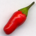
Above two lights are compared by the narrow-band components of their tristimulus vectors. At right the same information is shown, but projected into the v₁-v₂ plane. The loss of red-green contrast is the main issue with lights of “poor color rendering,” and that shows up in this flat graph. If you were really designing lights, you might use the v₁-v₂ projection as a main tool. You might want to add wavelength labels to the vectors.
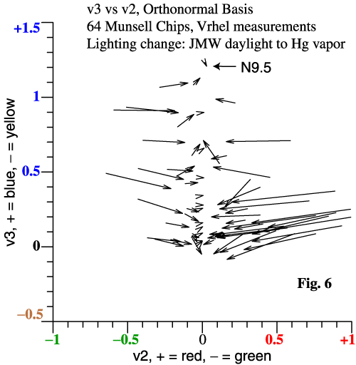
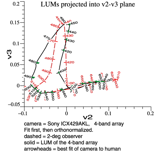
Other interesting data can be plotted in Cohen’s space. Suppose that the 64 Munsell chips from Vrhel et al. are illuminated first by daylight and then by the mercury light. Since the mercury light lacks red and green, we expect it to create a general loss of red-green contrast among the 64 chips. The graph at right is a projection into the v2-v3 plane. Each arrow tail is the tristimulus vector of a paint chip under daylight. The arrowhead is the same chip under the mercury light. The lightest neutral paper is N9.5, and is a proxy for the lights. Notice that 3-vectors projected into a plane still have the properties of vectors in the 2D plane. As expected, red and green paint chips suffer a tremendous crash towards neutral. [Michael J Vrhel, Ron Gershon, LS Iwan, "Measurement and analysis of object reflectance spectra.," Color Res. Appl. 1994;19:4–9.]
Actual neutral papers appear as arrows of zero length. For an alternate presentation about comparing lights, please see “How White Light Works,” and the related graphical material.

Cameras and the "Maxwell-Ives Criterion"

In 1889, Herbert Ives's father, Frederic Eugene Ives, stated the Maxwell-Ives Criterion: A color camera should have the same sensitivity functions as the eye. A Modern statement of the same idea: For color fidelity, a camera’s spectral sensitivities must be linear combinations of those for the eye.
For instance, in Fig. 1, (mini version at right), if one of the graphs represented a camera, it would meet the criterion. If a camera departs from the ideal, it is less obvious how to describe that situation. Some find a "figure of merit," but that gives little information. So, remember the invariant Locus of Unit Monochromats, LUM. The eye has an invariant LUM, and so does the camera.

One Stumbling Block

There is one stumbling block.
The LUMs may be similar or identical as shapes floating in space.
To compare them, we need to rotate them into good alignment.
The Fit First Method creates good alignment.

Compare Camera LUM to that of Human

At right is a screen grab from the virtual reality comparison of a Dalsa 575 sensor’s LUM to the 2° human observer LUM. The spheres represent the LUM of the camera The arrowheads trace the best fit to the human LUM by the camera functions.

Please let go of the details for a second, and try to see the big picture.

The human LUM is an invariant representation of trichromatic color vision. The camera has its own LUM. We want to compare them, but must somehow position them for a clear comparison. The Fit First Method finds the camera LUM in a good alignment.

The Fit First Method

Conceptually, the camera’s LUM (spheres) is more fundamental than the fit to the human LUM (arrowheads). The trick of the Fit First Method is to find the best fit first, then find the LUM from that. Here is the computer code: Rcam = RCohen(rgbSens) # 1 CamTemp = RcamOrthoBasis # 2 GramSchmidt(CamTemp, CamOmega) # 3 The camera’s 3 λ sensitivities are stored as the columns of array rgbSens . Because of the invariance of projection matrix R, it doesn’t matter how the functions are normalized, or whether they are actually in sequence r, g, b. Statement 1 finds Rcam, the projection matrix R for the camera. RCohen() is a small function, but conceptually, RCohen(A) = Ainv(A’A)A’ . (7) In other words, step 1 applies Cohen’s formula for the projection matrix. Then Rcam is the projection matrix for the camera. In step 2, the columns of OrthoBasis are the human orthonormal basis, Ω . The matrix product Rcam*OrthoBasis finds the projection of the human basis into the vector space of the camera. But, the wording about projection is another way of saying that step 2 finds the best fit to each ω_i by a linear combination of the camera functions. So, step 2 is the “fit” step. (More programming specifics.)
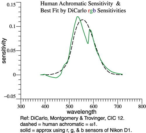
Step 2 does 3 fits at once, but let's look at just one. At right, the dashed curve is ω₁, the human achromatic function. The camera in question happens to be a Nikon D1. The solid curve is a linear combination of that camera’s r, g, and b functions that is the least-squares best fit to ω₁. There would be other ways to solve the curve-fitting problem, but projection matrix R is convenient. A best fit is found for each ω_j separately. The resulting re-mixed camera functions are not an orthonormal set.
Step 3, Orthonormalize the Re-mixed Camera Functions
Since the re-mixed camera functions are computed separately, they are not orthonormal and would not combine to map out a true Locus of Unit Monochromats. But they mimic Ω and are in the right sequence. We need to make them orthonormal, which is what the Gram-Schmidt method does, Step 3.

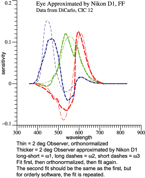
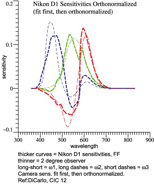The two sets of graphs above look similar. But the one on the left shows the set of “fit” functions. The one on the right shows the orthonormal basis of the Nikon D1. The thinner curves pertain to the 2° observer, the thicker ones to the camera. Why Does it Matter? When you have the orthonormal basis, for the eye or for a camera, you can do many things with it. Combining the 3 functions generates the Locus of Unit Monochromats. The orthonormal property leads to some simple derivations. On the Q&A page, see "Can we have fun with orthonormal functions?"

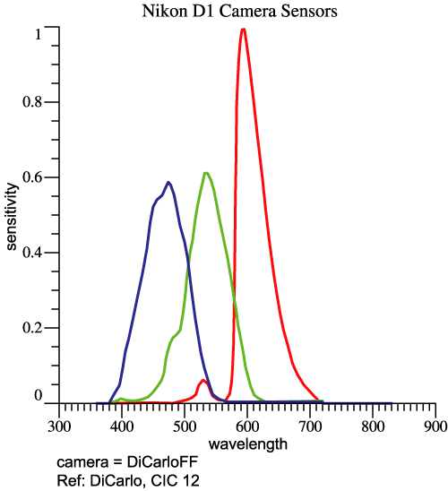
Camera Example, Nikon D1

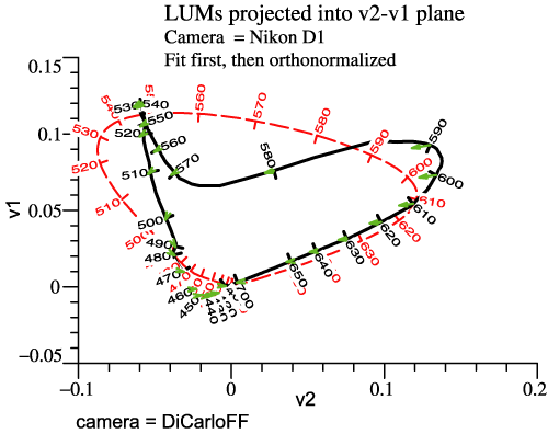
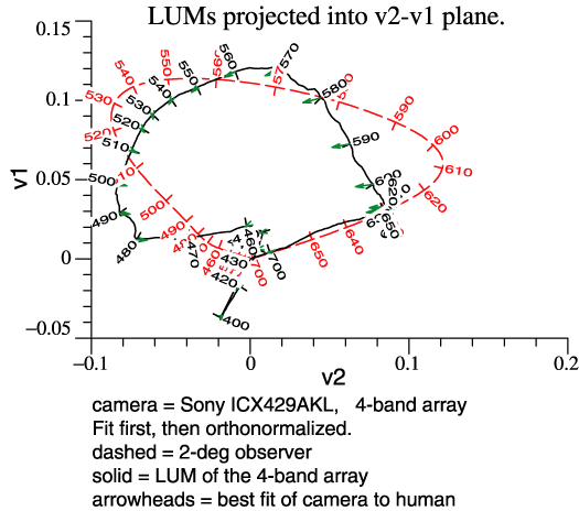
The last 4 graphs above pertained to the Nikon D1, based on data from CIC 12. At right are the camera’s red, green, and blue sensitivities. The camera’s LUM can be compared to the eye’s. Rather than another perspective picture, we now view the LUMs in orthographic projection (2 graphs below). The dashed curves are the human locus. The solid curves are the camera’s locus, while the tips of the small green arrows are points on the best-fit sensitivity function.

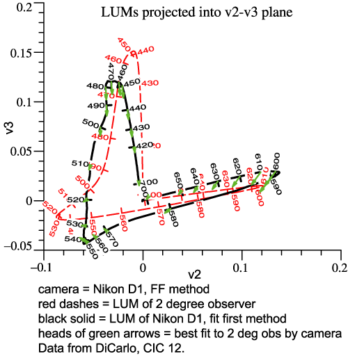Now you may say “These curves mean nothing to me!” That may be true at first, but the graphs contain a complete description of the camera sensor, with no hidden assumptions, and no information discarded. Finding Some Meaning in the Camera's LUM Consider the left-hand graph, “LUMs projected into v2-v1 plane.” Only the red and green receptors contribute to the human LUM in this view, and v1 is the achromatic dimension for human, based on good old y-bar. In this plane at least, the particular camera tends to confuse wavelengths in the interval 510 to 560 nm, which are nicely spread out as stimuli for human. Yellows, say 560 to 580 nm, have lower whiteness than they would for human. The camera has other differences from human that may be harder to verbalize. To the extent that finished photos look wrong, one could revisit these graphs for insight. More Examples Five detailed examples were prepared in 2006, and they are linked from the further examples page. For instance, Quan’s optimal sensor set indeed looks good in any of the graphical comparisons to 2° observer. (See http://www.cis.rit.edu/mcsl/research/PDFs/Quan.pdf .)

Skip to End

Skip to Joe Photo

Something Completely Different: a 4-band Array

Nominal time: 3:08 pm

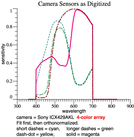
Sony publishes a specification for a 4-band sensor array, the ICX429AKL. I’m not sure of the intended application, but it could potentially be applied in a normal trichromatic camera. The Fit First Method readily fits the 4 sensors to the 3-function orthonormal basis.
The four sensitivities are seen at right. The key steps look the same: Rcam = RCohen(rgbSens) CamTemp = Rcam*OrthoBasis GramSchmidt(CamTemp, CamOmega) . Recall that the projection matrix Rcam is a big square matrix of dimension N×N, where N is the number of wavelengths, which might be 471. The 4th sensor adds a column to the array rgbSens, but does not change the dimensions of the result Rcam. After the key "fit first" steps, I did have to re-think some auxiliary calculations because of the 4-column sensor matrix.
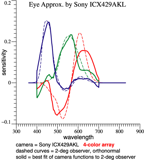
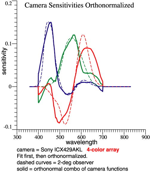
The camera's orthonormal basis Rcam comprises 3 vectors that are linear combinations of the 4 vectors in rgbSens. I wanted to find the 4x3 transformation matrix relating the one to the other, in order to stimulate thinking about noise. The program output itself explains the method as follows: Similar to Eqs. 15-18 in CIC 14 paper, Transform from sensors to CamOmega: We want to solve CamOmega = rgbSens * Y , where Y is coeffs for 3 lin. combs. MPP = inv(rgbSens'rgbSens) rgbSens' Y = MPP*CamOmega = 0.24845 0.13737 0.35971 -0.34663 -0.43708 -0.45585 -0.22433 -0.088434 -0.033503 0.26839 0.22522 0.055984 Column amplitudes = vector lgth of each column = 0.55158 0.51812 0.58433 The columns of rgbSens actually contain the 4 sensitivities, cyan, green, yellow, magenta. MPP is the Moore-Penrose Pseudoinverse. (See Wikipedia and pp. 9-10 in "notes.") Keeping in mind that the sensitivities are all >= 0, matrix Y gives some idea how much subtraction is done to produce the sensor chip’s orthonormal basis. That’s a step toward thinking about noise. Below are the 3 orthonormal functions, and also the 3 best-fit functions made from the 4 camera sensitivities. The only source of “noise” is the errors that I introduced while converting graphs to numbers. It becomes more visible here, after subtractions.

Some noise also shows up in the projections of the LUM, below. It would appear that color fidelity is not good; reds and oranges may lose some redness.

Combining LEDs to Make a White Light?

In the 1970s, William A. Thornton asked an interesting question: If you would make a white light from 3 narrow bands, how would the choice of wavelengths affect vision of object colors under the light? His research led to the Prime Colors, a set of wavelengths that reveal colors well. From that start, he invented 3-band lamps and was named Inventor of the Year in 1979. 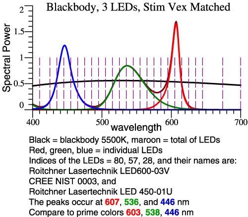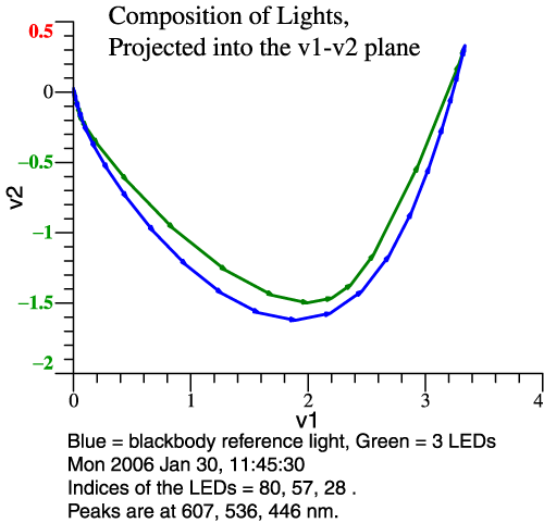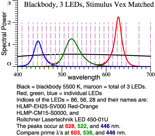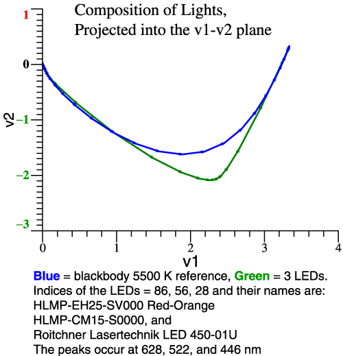He continued his research and made the definition of prime colors more precise. Problem Statement: For the 2° Observer, Thornton’s Prime Colors are 603, 538, 446 nm. [See CIC 6, and Michael H. Brill and James A. Worthey, "Color Matching Functions When One Primary Wavelength is Changed," Color Research and Application, 32(1):22-24 (2007). Also see Wavelengths of Strong Action, above.] If you would make a light with 3 narrow bands at those wavelengths, the light would tend to enhance red-green contrasts, making some colors more vivid, though it would do a bad job with saturated red objects. You might think then that a white light could be made from 3 LEDs whose SPDs peak at those wavelengths. This idea falls short because LEDs are not narrow-band lights. Our task then is to see what happens when real LEDs are combined, and design a good combination by speedy trial-and-error. We'll see two graphs per example: the LED spectra and their sum, and then the vectorial composition of the LED light in comparison to 5500 K blackbody. Clicking either image gives more detailed information. Example 1: Let LED Peaks ≈ Prime Colors The reference white is 5500 Kelvin blackbody. From 119 types measured by Irena Fryc, 3 LEDs are chosen by their peak wavelengths, as shown at left. Then we see at right that the blackbody (blue line) makes a bigger swing to green and back. This LED combo will dull most reds and greens.

Example 2: Greener Green and Redder Red To increase the swing towards green and back, we let the green be greener (shorter λ) and the red be redder (longer λ). In all cases, the LED amplitudes are adjusted so the total tristimulus vector matches the blackbody.

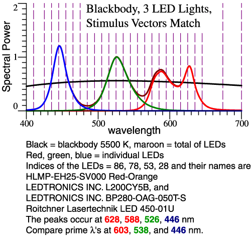
Still on example 2, we can see from the vector composition (right-hand graph) that red-green contrast will be good, but some colors may be particularly distorted. Clicking the left-hand graph confirms that idea in the color shifts of the 64 Munsell papers. Example 3: Broaden the Red Peak The problem in example 2 is known to some lighting experts. The light needs to have a broader range of reds. The remedy is to use 2 red LEDs. For simplicity, the proportion of the 2 reds is fixed, not adjustable.

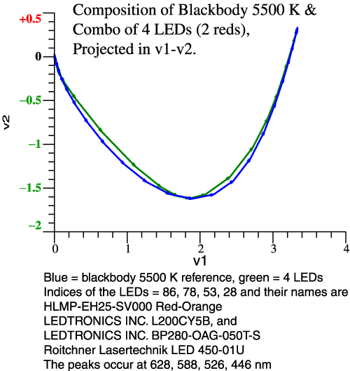Think of those green and red limit colors. Some of those colors will still be dulled, but we are tracking the blackbody pretty close. Further tweaking is possible.

3:22 pm

Vectorial Color

Sets of functions can be equivalent for color matching, but look different, and have other meanings, such as cone sensitivities or opponent functions, Fig. 1. This great insight is part of our legacy from the 20th century and earlier.
But, which color matching functions are best for graphing color vectors? There is no 20th-century answer, but you can take Guth’s 1980 functions, and orthonormalize them, and that will work. That’s the orthonormal basis.
Jozef Cohen noticed that colors have intrinsic vector relationships. His work led to the invariant Locus of Unit Monochromats.
In its original use, Cohen’s projection matrix R takes any spectral power distribution and finds a metamer that is a linear combination of the color matching functions used to make R.
More generally, R can be used to fit any function by a linear combination of functions. Using R in this way leads to the 3-step Fit First Method for finding a camera’s Locus of Unit Monochromats.
We have analyzed lights and cameras. The graphical methods tend to preserve details, not lose them.
Matrix R and the orthonormal basis lead to interesting algebraic methods. See the Q&A page.
In making vector diagrams, you'll find that you must adjust a vector length, or adjust two vectors to match, and so forth. If those steps feel unfamiliar, it's because traditional methods tend to discard the amplitude of color vectors.

Invariants

My numbers and graphs are based on the 2º observer. If a different standard observer were used, details could change, but certain basic ideas would not change:

The formula for R:

R = A(A^TA)^-1A^T . (10)

The fact that R is always the same numerical array, for a given observer.
The relationship of R to the orthonormal basis:

Ω^TΩ = I_3×3 . (15)
ΩΩ^T = R . (16)

The LUM for the 2º observer, including the wavelengths of the longest vectors. Plotting the rows of Ω draws the LUM. A different orthonormal basis for the 2º observer will draw the same LUM.
The fact of red-green overlap, and the implication that a light can be deficient in red and deficient in green.
The idea that a camera has an LUM, and if its LUM is the same as the eye’s, then the camera meets the Maxwell-Ives criterion.

If vectorial color is forgotten and then re-invented in 50 years, these ideas will come out the same. They transcend the personalities of those who discovered them.

Food for Thought ...

Vectorial Color Is About Color Mixing.
It Is Not About Any Neural Processing, Only Transduction.

Cohen’s ideas relate to making best use of color mixing data. The orthonormal CMFs are a convenient way to map stimuli into the invariant color space. They are not a hypothesis about retinal wiring.

We have also seen that "mere" color mixing—the linear stage of vision—is the key to understanding color rendering and color camera sensors.

The End

Please feel free to contact me at any time. I am always

eager to discuss lighting, color, cameras etc.

Jim Worthey

www.jimworthey.com

Special Credit

William A. Thornton
Jozef B. Cohen

Michael H. Brill
Tom Cornsweet (1970 Book)
Ronald W. Everson (taught color fundamentals)
David MacAdam and Gershon Buchsbaum who mentioned orthogonal color matching functions.

(But MacAdam gets a demerit for disparaging Cohen's work.)

Calculations were done with O-matrix software.

William A. Thornton
1923-2006

Jozef B. Cohen
1921-1995

Bonus Picture: Jim Worthey, Jozef Cohen, Nick Worthey, circa 1993
Jim, Jozef, Nick

Stop

Scroll No Farther

Material Below Addresses Obscure Questions

Spectrum Locus for 4 Different Sets of Color Matching Functions

Orthonormal Basis Functions (Graph as Cohen drew it.)	Color Matching functions similar to Raw Experimental Data
Cone sensitivities, r, g, b	CIE's x-bar, y-bar, z-bar

"Boomerang Graph," Not a Chromaticity Plot